
Recall that in our last post, we had ablated various training and rollout parameters to maximize performance. We were after a particular use case – we had a pristine dataset collected on a YAM data collection rig and we wanted to roll a model trained on that rig onto another slightly different, but still YAM-based setup.
Part of the reason was selfish – we wanted to be able to do model demos without freighting an entire mobile rig around (it doesn’t pack very well). But it seemed to be a useful thing to understand for our research partners and smaller customers doing mid/post-training on our data: a big lab will just duplicate the rig from CAD, but a smaller lab might have an existing setup they want to use.
We had discovered that matching the gross camera intrinsics such as field of view were a good idea, that you should probably train the expert and the backbone, and that lighting, as expected, was a big factor. We also discovered that the model is very sensitive to arm intrinsics; a well-worn or poorly-zeroed arm with a couple of degrees of cumulative offset in the encoders was enough to drop accuracy to nearly zero.
The Latency Bug
After carefully matching the cameras, burning something like 1000 GPU-hours to train many checkpoints (wow, aren’t we glad we have an in-house training rig!), ablating 10K runs in sim to chase bugs, and triple checking the arms weren’t zeroed improperly, we were greeted with…less performance than we liked. At this point we were ready to cave in and do a final RL pass to learn what we thought were deviant rig intrinsics on the rollout hardware, but fortuitously, one of us had the intelligence to go watch the video feed in the inference dashboard.
Why fortuitous? Well, usually the guy tending to the rollout is supposed to watch the arms with a hand over the e-stop, not the WebUI. In any case, it quickly became clear there was several hundred milliseconds of latency in the video feed – earlier, we had just sort of ignored it because we figured it was some Web thing (web video protocols usually default to a 1s+ buffer to absorb network variations).
Investigating the latency revealed it was real and a result of an unfortunate Python quirk – Python’s buffered pipe was waiting for 64 KB of frames to accumulate before making them accessible and at the tiny frame size the inference code was using this was quite a few frames. We patched out the latency and performance markedly improved – in particular, we previously had unexplainable bias in first approaches during “pick” and similar bias during “place”. It also revealed…
A Sim-to-Real Gap
We were pretty satisfied with our in-house simulator, which was crafted with just enough physics to be a good diagnostic tool. As part of the 10K+ ablations, we had ablated latency, concluding that up to 280 ms of latency was inconsequential to all aspects of model accuracy – this was one of the reasons we didn’t find the extra latency earlier, because we weren’t looking for it.
Evidently, the simulator was lying, because removing a similar amount of latency in the real system had a huge effect on performance. Our first theory was that injecting vision latency was different from injecting inference latency, so we went and did another 1000 runs on varying amounts of vision latency – the sim showed the same behavior, namely almost no change.
Our standing theory is that the extra latency increased the number of near misses, which causes collateral damage in the scene. The collateral damage is hard to simulate – there are a lot of damped collisions, the containers can tilt, and objects can roll or slide with varying degrees of friction. The sim used a simple physics model that masked a lot of this damage, but in the real setup objects would go flying or rolling on a bad run. Compounding this was objects far from the work area being out of distribution, which would trigger erratic actions that tended to knock the remaining targets around even more. Finally, perceived performance can differ from benchmark scores – in the same way that LLMs can benchmark high but be terrible in practice, a VLA can “usually” complete the task but do so in an unpleasant way.
Optimizing the Inference Engine
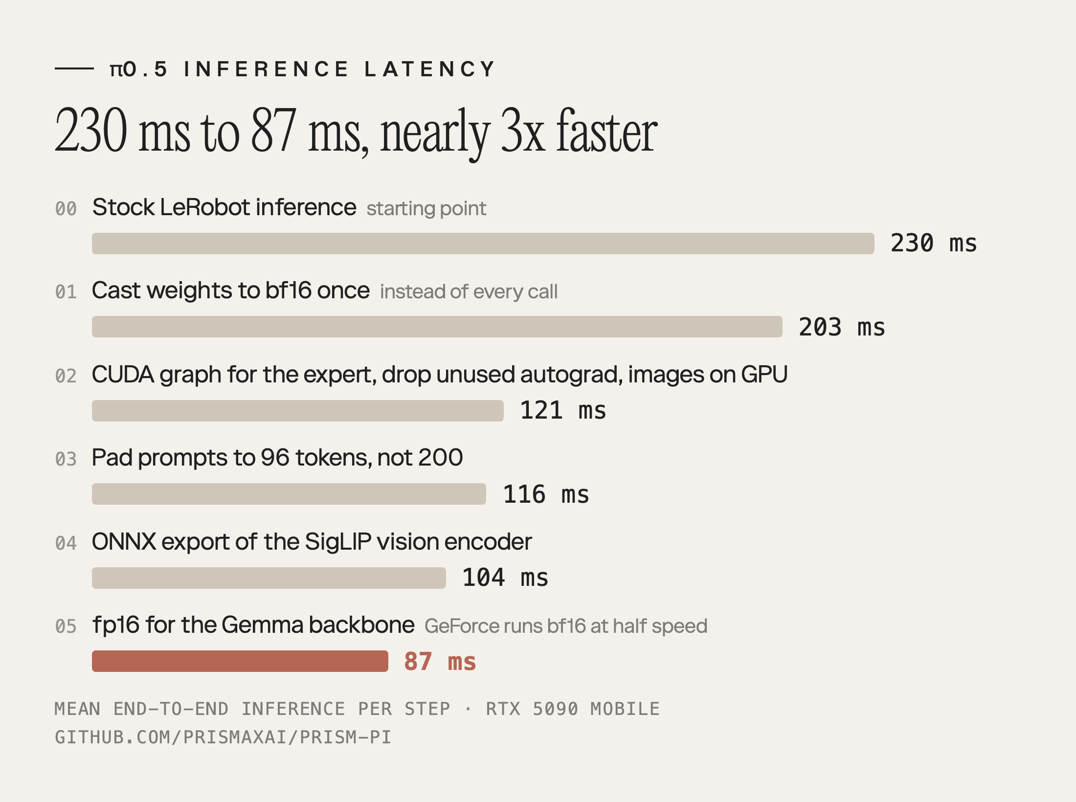
As part of the initial latency chase, we noticed that while knocking off 100+ ms of buffer latency only slightly improved performance, knocking off another 90 ms of camera latency (this camera seemed to have four frames of latency, so running at 120 Hz greatly reduced it) gave a much bigger jump. As we had over 230 ms of mean inference latency from the stock LeRobot codes, we were excited to see whether shaving this number down would give us even more performance gains.
It’s a bizarre fact that despite being the most performance-sensitive field of computer science to show up since video games were invented, off-the-shelf AI code tends to be pathologically slow in the stupidest of ways. Case in point: we saved 25 ms (10%!) by simply converting the weights to bf16 in the beginning instead of once every call, because for some reason Hugging Face codes love to store things in fp32. This shaved step time to about 203 ms.
We then discovered that the 10 action generation steps took a total of 86 ms, most of which was spent doing very little. Capturing a CUDA graph of the expert dropped that down to 17 ms. We also discovered a bug, costing us 35 ms, where an autograd graph was being recorded for the whole model but never used. Moving image conversion to the GPU saved us another few ms, bringing down the end-to-end inference latency to 121 ms.
We were padding prompts to 200 tokens, but our prompts were simple, short task tags. Shaving this down to 96 tokens netted us another 5 ms, which is palpable when the entire pass is only 121 ms. We then built an ONNX export for the SigLIP vision encoder, which knocked out another 12 ms – not much, but that’s 10% at 121 ms per step.
We attempted to export an ONNX version of the rest of the Gemma backbone but only got 10 ms improvement. We were puzzled – normally ONNX is good for 2x on an LLM-shaped model – until we remembered that the RTX 5090 Mobile we were running on was limited to half-speed bf16. Swapping over to fp16 (and carefully watching for NaNs) got us all the way down to 25 ms for Gemma. This brought end-to-end latency down to 87 ms, nearly 3x faster than we had started.
Did It Matter?
Yes! With end-to-end latency down to under 120 ms we were able to observe emergent behavior in the model matching the training data. In particular, our human operators would often do a fast approach, followed by a pause to gauge gripper position and a small correction before the grab. With the latency shaved down, we were able to see this behavior reflected in the rollout. We also observed other emergent behavior such as cross-handed placement and hand swaps in one session, which we had also incorporated sparingly into the training dataset.
The code is open source as prism-pi – you could reproduce our results with a few Claude Code prompts from the existing LeRobot codebase, but we’ve found that having a reference for your agent to work on that someone else already tested still helps accelerate development. With a fast camera and a desktop RTX 5090, this code should be able to achieve sub-50 ms latency, which is solidly realtime. Enjoy!